Rmongodb Package In R Download

R is a powerful and popular language for statistical analysis, modeling, and visualization. MongoDB offers powerful querying features for fast retrieval and analysis of big data, and its flexible schema makes it a natural choice for unstructured datasets. By connecting MongoDB and R, we can perform advanced data analytics in no time using the MongoDB aggregation pipeline.

Read on to learn more about R MongoDB drivers and get started using them for data analysis.

Getting Started with MongoDB in R

To install R, download the relevant package for your operating system from the CRAN downloads page.

You can then install and use the latest version of RStudio to view the results and visualizations all in one place.

You'll also need to be running MongoDB. We recommend you try the MongoDB Atlas free-tier cluster for this tutorial. MongoDB Atlas is easy to set up and has sample datasets for R MongoDB examples. You can load sample datasets using the "…" next to the collections button on your cluster page.

R Packages for MongoDB

You'll need a MongoDB client to establish a reliable MongoDB connection in R. The preferred R MongoDB driver, mongolite, is fast and has a syntax similar to that of the MongoDB shell. mongolite is the one that will be used in the following examples. The other packages listed here haven't been as active on Github recently. The most popular packages to connect MongoDB and R are:

• mongolite: A more recent R MongoDB driver, mongolite can perform various operations like indexing, aggregation pipelines, TLS encryption, and SASL authentication, among others. It's based on the jsonlite package for R and mongo-c-driver. We can install mongolite from CRAN or from RStudio (explained in a later section).

• RMongo: RMongo was the first R MongoDB driver with a simple R MongoDB interface. It has syntax like the MongoDB shell. RMongo has been deprecated as of now.

• rmongodb: rmongodb has functions to create pipelines, handle BSON objects, etc. Its syntax is very complex compared to mongolite. Just like RMongo, rmongodb has been deprecated and is not available or maintained on CRAN.

How to Connect to a MongoDB Database in R

There are several sample datasets available in the MongoDB Atlas free cluster. You will use the sample_training database as it contains many collections suitable for data analysis with R.

Open RStudio (or any IDE/editor of your choice). Create a new document with the name trips_collection.R. You can create a separate file for each collection used in this tutorial (refer to github repository).

Install mongolite by running the following in the newly created file (or console if you are using RStudio) as:

          install.packages("mongolite")        

Then, load it using the command:

          library(mongolite)        

Next, connect to MongoDB and retrieve the collection using the mongo() function in the R code to get the trips collection from the sample_training database. This collection contains data from trips executed by the users of a bike share service based in New-York City.

          # This is the connection_string. You can get the exact url from your MongoDB cluster screen connection_string = 'mongodb+srv://<username>:<password>@<cluster-name>.mongodb.net/sample_training' trips_collection = mongo(collection="trips", db="sample_training", url=connection_string)        

You can verify that your code is now connected to the MongoDB collection by checking the total number of documents in this database. To do so, use the count() method.

          > trips_collection$count() [1] 10000        

Now that you have a connection established to the database, you will be able to read data from it to be processed by R.

How to Get Data into R from MongoDB

In this section, you will learn how to retrieve data from MongoDB and display the same. Let's continue with the trips_collection from the previous section.

You can use the MongoDB Atlas UI to view the trip_collection documents, or RStudio to visualize it.

Get any one sample document of the collection using the $iterate()$one() method to examine the structure of the data of this collection.

          > trips_collection$iterate()$one()  $tripduration [1] 379 ...        

Now that you know the structure of the documents, you can do more advanced queries, such as finding the five longest rides from the trips collection data. And then listing the duration in descending order.

          > trips_collection$find(sort = '{"tripduration" : -1}' , limit = 5, fields = '{"_id" : true, "tripduration" : true}')                        _id tripduration 1 572bb8222b288919b68ac07c       326222 2 572bb8232b288919b68b0f0d       279620 3 572bb8232b288919b68b0593       173357 4 572bb8232b288919b68ae9ee       152023 5 572bb8222b288919b68ac1f0       146099        

The above query uses sort and limit operators to produce this result set.

How to Analyze MongoDB Data in R

To analyze MongoDB with R in more detail, you can use the MongoDB aggregation framework. This framework allows operators to create aggregation pipelines that help in getting the exact data with a single query.

Suppose you want to check how many subscribers took trips of a duration >500 seconds and returned to the same station where they started. The query uses MongoDB $expr (expressions) to compare two fields in the same document.

          query = trips_collection$find('{"usertype":"Subscriber","tripduration":{"$gt":500},"$expr": {"$eq": ["$start station name","$end station name"]}}')  # Get number of records using nrow method nrow(query) [1] 97        

Combining these operators with some R code, you can also see which type of users are more common: subscribers or one-time customers. To do this, group users by usertype field.

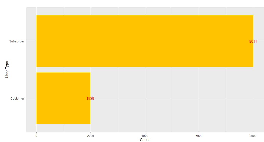
          user_types = trips_collection$aggregate('[{"$group":{"_id":"$usertype", "Count": {"$sum":1}}}]')        

To compare the results, you can visualize the data. It's convenient to convert the data obtained from mongolite into a dataframe and use ggplot2 for plotting.

          df <- as.data.frame(user_types)  install.packages("tidyverse", dependencies=T) install.packages("lubridate")  install.packages("ggplot2") library(tidyverse) library(lubridate) library(ggplot2)  ggplot(df,aes(x=reorder(`_id`,Count),y=Count))+ geom_bar(stat="identity",color='yellow',fill='#FFC300')+geom_text(aes(label = Count), color = "red") +coord_flip()+xlab("User Type")        

You should see the following plot in RStudio:

Let's explore another bar plot with a different collection — inspections. This collection contains data about New York City building inspections and whether they pass or not. For the following examples, start with a new file named inspections_collection.R.

          inspections_collection = mongo(collection="inspections", db="sample_training", url=connection_string)        

Suppose you want to check the number of companies that failed inspections in 2015 versus 2016.

If you view the data in the Atlas UI, you will notice that the date field is a String. To convert it into date type and then extract the year will require some processing— or so you would think. But, with the Mongodb aggregation pipeline, you can do everything in a single query. For manipulating the date field, use the $addFields operator.

          year_failures = inspections_collection$aggregate('[{"$addFields": {"format_year":{"$year":{"$toDate":"$date"}}}}, {"$match":{"result":"Fail"}}, {"$group":{"_id":"$format_year", "Failed": {"$sum":1}}}]')        

You are grouping the results by year, so it's easy to create a plot:

          df<-as.data.frame(year_failures)  ggplot(df,aes(x=reorder(`_id`,Failed),y=Failed))+ geom_bar(stat="identity", width=0.4, color='skyblue',fill='skyblue')+ geom_text(aes(label = Failed), color = "black") +coord_flip()+xlab("Year")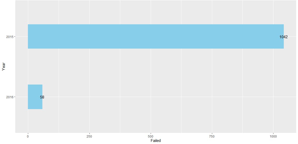        

You can see this new chart in RStudio. Using the aggregation framework made it easy to extract the data from the database and structure it in a way that was easy for R to plot in our chart.

Next, let's create a line plot. Let's use the companies collection, which contains information about companies such as their foundation year and their headquarter addresses. To explore this dataset, create a new file companies_collections.R.

Say you want to know the trend of the number of companies with category_code = 'consulting' founded after 2003. For this, use the relational operator $gt, group the results by founded_year and sort them to be displayed in the line plot. Again, this can be done in a single query.

          companies_collection = mongo(collection="companies", db="sample_training", url=connection_string)  consulting_companies_year_wise = companies_collection$aggregate('[ {"$match":{"category_code":"consulting","founded_year":{"$gt":2003}}}, {"$group":{"_id":"$founded_year", "Count": {"$sum":1}}}, {"$sort":{"_id": 1}} ]')  df<-as.data.frame(consulting_companies_year_wise)  ggplot(df,aes(x=`_id`,y=Count))+ geom_line(size=2,color="blue")+ geom_point(size=4,color="red")+ ylab("Number of consulting companies")+ggtitle("Year-wise (2004 onwards) companies founded in the category 'consulting'")+xlab("Year")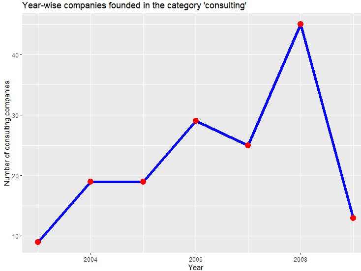        

You can see a steady increase in the number of consulting companies until 2008, after which there is a steep decline. Once again, using the aggregation framework made it easy to transform the data in a format ready to be used with R.

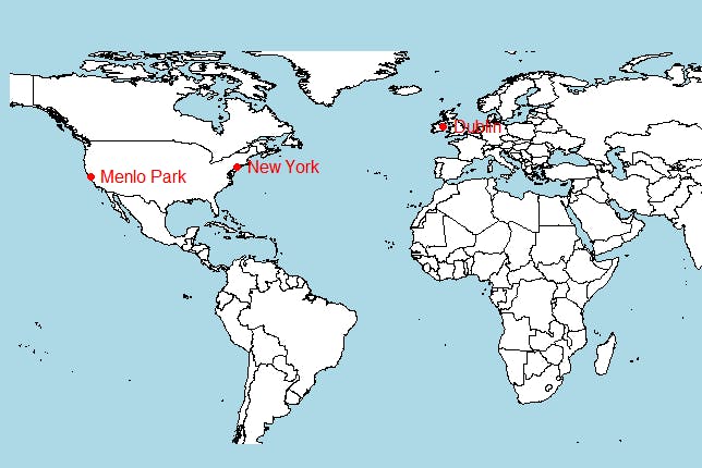
You can also create maps from data received from MongoDB. Let's find all the office locations of the company named Facebook. Note that the offices field is an array with many objects having fields like city, latitude, and longitude. To retrieve individual objects and fields, use the $unwind aggregation operator— another operator that can get most complex objects in a simpler form to extract data in an efficient way.

          # Get the location array objects fb_locs = companies_collection$aggregate('[{"$match":{"name":"Facebook"}},{"$unwind":{"path":"$offices"}}]')   # Get individual fields from each array object loc_long <- fb_locs$offices$longitude loc_lat <- fb_locs$offices$latitude loc_city <- fb_locs$offices$city  # Plot the map install.packages("maps") library(maps)  map("world", fill=TRUE, col="white", bg="lightblue", ylim=c(-60, 90), mar=c(0,0,0,0)) points(loc_long,loc_lat, col="red", pch=16) text(loc_long, y = loc_lat, loc_city, pos = 4, col="red")        

For more advanced analytics, you can use sophisticated APIs like ggmap as well. Since this is a simple display, use the basic map() function.

MongoDB and R allow you to perform different types of analytics. R is also popular for extracting statistics from data. To understand that, let's use the grades collection which contains information about grades of students for a set of assignments. Create a new file grades_collection.R where you will load this collection.

          grades_collection = mongo(collection="grades", db="sample_training", url=connection_string)        

Let's get the average of all the scores of all the students who attended the class with id 7. Use $project to get only specific fields.

          class_score_allstudents = grades_collection$aggregate('[{"$match":{"class_id":7}},{"$unwind":{"path": "$scores"}},{"$project":{"scores.score":1,"_id":0,"scores.type":1,"class_id":1}}]')        

The scores field is an object which has a type and score fields. You can extract all the score values into a single vector:

          score_values <- class_score_allstudents$scores$score        

R provides us with many tools to manipulate the data from those grades. Get the median and mean of the class using statistical functions:

          > median(score_values) [1] 49.96923  > mean(score_values) [1] 50.80008        

You can get the same information and more using a box and whisker plot:

          b<-boxplot(score_values,col="orange",main = "Overall score details of all students attending class with id '7'")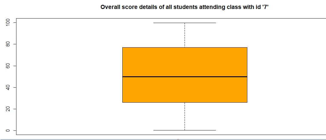        

You can add all the data points using the stripchart function:

          stripchart(score_values, method = "jitter", pch = 19, add = TRUE, col = "black", vertical=TRUE)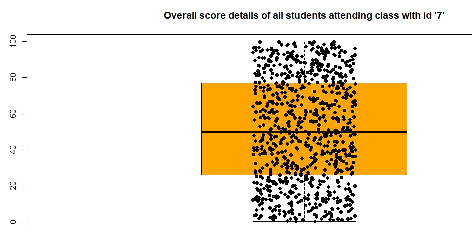        

View the same statistics on the console using the $stats function:

          > b$stats            [,1] [1,]  0.1798022 [2,] 25.9990090 [3,] 49.9692287 [4,] 77.0596579 [5,] 99.9447486 >        

You can also plot a histogram to see the ranges of scores of students of class_id 7 in the exam:

          # Get the scores array student_score_exam = grades_collection$aggregate('[{"$unwind":{"path": "$scores"}},{"$match":{"class_id":7,"scores.type":"exam"}}]')  # Get the score values for 'exam' field for all the students scores_of_allstudents <- student_score_exam$scores$score hist(scores_of_allstudents,col="skyblue",border="black",xlab="Scores of all students of class id 7")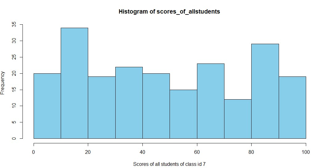        

To view the range (min and max values) and all the data points, use the R functions range() and sort() respectively:

          sort(scores_of_allstudents)  range_scores = range(scores_of_allstudents) [1]  0.2427541 98.6759967        

You can perform a lot of complex manipulations and data analysis using MongoDB and R. You can try a few more now that you have the datasets and hands-on experience.

Posted by: falseessence.blogspot.com

Source: https://www.mongodb.com/languages/mongodb-and-r-example